The programs are a javascript version of C programs that are made by Joey de Vries and are part of the website www.learnOpenGL.com (On the site is a menu with the opetion 'Code Repository'. In the same menu is an option 'Offline book'. The chapters in this file refer to that book).
No comments
To get a time value we have used performance.now(). The function returns time in mili-seconds. To get a decent value we divided by 1000.
The creation code for a shader is now in a seperate file in the subdirectory /common. We are not reading the shader code from file. Instead we put the shader code as a java variable in an include file. The files are in the subdirectory /js/ChX/shaders. And we add an extra file index.js to this directory from which all the variables with shader code are exported.
The book uses a library to load textures. We replace it with loading an Image and using this as the texture source. Loading of an image is not synchronous. Before it is loaded the texture is made a 1x1 blue pixel. For producing this pixel the function InitTexture() is made. Now we need the requestAnimationFrame() in the render() if we do not add a requestAnimationFrame() after the load of the image. Otherwise we see only a blue texture.
In this chapter we need a math library. There are many. We choose on that has many users and also has support for Quaternions (needed for interpolation of rotations): gl-matrix. It can be downloaded from npm using 'npm i gl-matrix' and it gets installed in the node_modules subdirectory. We use version 3.3. We will only use the esm (Ecma script modules) version and have copied the classes from the gl-matrix/esm subdirectory in node_modules to the projectXXX/math/glmatrix subdirectory and next deleted the gl-matrix/esm subdirecory in node_modules. Note that the subdirectory also has the index.d.ts type definitions. The syntax of the math is different from the usual. No operator overloading for instance. Create matrices with Mat4.Create(), vectors with vecX.fromValues(...). Changing matrices is done by using the matrix as input and output matrix, e.g. `Mat4.Translate(myMatrix, myMatrix, Vec3.fromValues(1.0, 1.0, 3.5)). When the internal format and format are different we get: GL_INVALID_OPERATION: Invalid combination of format, type and internalFormat (gl.RGB and gl.RGBA).
We have a real 3d object in this program, a cube. There are many libs with geometry objects like cubes, planes, spheres and more. In the program we make use of the depth buffer. And we have a combination of projection view and model matrices. Our Shader class has no method to set uniform matrices or vectors.
A camera class is created. Note that the projection matrix is not part of the class although the Zoom field does make part of it. The Zoom field is updated with the mouse scroll. The class KeyInput and Mouse are added to the common directory. We will be using the same constants for the keys as are used in the glfw library, like GLFW_KEY_W for the 'w' key etc.
The camera we use is based on the one given in the LearnOpenGL book. It uses a Pitch-Yaw-Roll camera for the orientation of the camera and a position field. The orientation is controlled by the mouse and the position by the WASD keys. Note that OpenGL uses degrees instead of radians to measure angles.
Let us call the coordinate axes of the world (XYZ) and the coordinate axes of the object (the camera) (xyz). The camera has its front in the direction -z! The up direction of the camera is y and the right is x. The start configuration of a camera is defined by its z-axis and by the up-direction in the world, Y. Its z-axes is in the opposite of the view-direction, the x-axes is z \(\times\) Y (using the outer product and Y: the world up axis), the y-axes is z \(\times\) x, creating a right handed system (xyz).
Now we have two coordinate systems and we can use both to define rotations around the axes, the axes of the world system and the axes of the camera, the local system. We will use the local system and assume that both systems are aligned with each other before any rotation has been made. By a theorem of Euler any orientation relative to the world system can be reached with three consecutive rotation around the axes. We could choose for a system where first we rotate around the X-axis, then around the Y-axis and then around the X-axis again as one of many choices. We will use a system that uses the local system with first a rotation around the y-axis (with the yaw-angle) then around the x-axis (with the pitch-angle) and finally around the z-axis (the roll angle).
Note that rotations in the world frame and local frame are related to each other. If we have \(R_Z(\alpha)\) stand for rotation of \(\alpha\) degrees in the local frame around the Z-axis, then we have \(R_Y(\gamma) R_X(\beta) R_Z(\alpha)\) = \(R_z(\alpha) R_x(\beta) R_y(\gamma)\), the rotations in the opposite order. Using only 2 rotations this can be seen by first writing \(R_x(\beta)R_y(\gamma)\) = \(R_x(\beta)R_Y(\gamma)\) because with the first rotation \(R_y\) there is no difference between local and world axes and then \(R_x(\beta)\) = \(R_Y(\gamma)R_X(\beta)R_Y(-\gamma)\), going back to the world frame, doing the rotation there and going back to the local frame.
In the book it is assumed there is no rotation around the Roll-axis. In updateCameraVectors() the Pitch-rotation and Yaw-rotation values are used to calculate a new orientation (a new XYZ), and GetViewMatrix() returns the new corresponding view matrix.
In the book there is a method to find after a rotation the new view matrix by first finding the z-axis in the rotated system. We can do this also by a calculation of the product of two rotation matrices, one for the pitch an one for the yaw:
\[\begin{equation*} \begin{pmatrix} cos(y) & 0 & sin(y) \\ 0 & 1 & 0 \\ -sin(y) & 0 & cos(y) \end{pmatrix} \quad \begin{pmatrix} 1 & 0 & 0 \\ 0 & cos(p) & -sin(p) \\ 0 & sin(p) & cos(p) \end{pmatrix} \quad \begin{pmatrix} 0 \\ 0 \\ 1 \end{pmatrix} = \begin{pmatrix} sin(y)cos(p) \\ -sin(p) \\ cos(p)cos(y) \end{pmatrix} \end{equation*}\]
Using \(sin(y) = cos(y-90)\) and \(cos(y)=-sin(y-90)\) and setting \(y^*=y-90\) the result is \((cos(y^*)cos(p), -sin(p),-cos(p)sin(y^*))\). We used counter clockwise angles as positive angles, when using clockwise angles the result becomes the same as the formula given in the book.
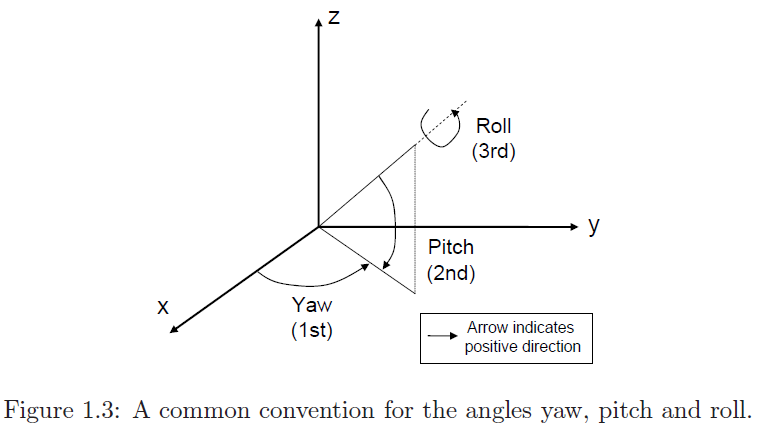
We have to be carefull when using formulas from others, because there are so many different parametrizations of rigid motion in 3D. As an example we have the following figure from an article that discusses transformations between different representations of rigid systems in robotics
They use the order yaw-pitch-roll with local rotations, as we do. But they use a different coordinate system. We think of the horizontal plane as being the ZX-plane, here it is the XY-plane. And also the angles are defined differently.