In chapter 43 of the book the theory of PBR, physics based rendering, is treated. The central formula is given as
\(L_o(p, \omega{_i}) = \int_\Omega f_r(p, \omega{_i}, \omega_o) L_i(p, \omega_i) (n.\omega_i) d\omega_i\)
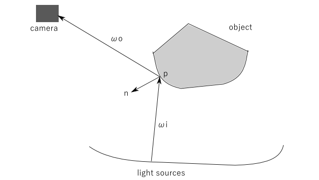
where L stands for the radiance and \(\omega_i\) and \(\omega_o\) stand for incoming and outgoing directions and n for a normal at the point p of the object. We have a small excercise on radiance and irradiance at te end of this file.
Many light sources might be present and of all kinds, sunlight, point lights, the environment map (IBL, image based lighting). When looking at the point p all those sources contribute, all having their own direction \(\omega_i\), to the ray going to the camera.
The \(f_r\) in our equation is split in two contributions, a diffuse and a specular one:
\(f_r = k_d.f_{lambert} +k_s.f_{cook torrance}\)
The \(f_{lambert}\) is in its simplest form the surface color c, \(f_{lambert}= c/\pi\). The \(f_{cooktorrence}\) is complicated and is the factor that expresses the dependency on the incoming and outgoing directions \(\omega_i\) and \(\omega_o\).
A formula for this is
\(f_{cooktorrance} = \frac{nDist.Fresnel.Geom}{4(\omega_0.n)(\omega_i.n)}\)
where - the Normal Distribution function approximates the amount the surface’s microfacets that are aligned to the halfway vector influenced by the roughness of the surface; this is the primary function approximating the microfacets. - the Geometry function describes the self-shadowing property of the microfacets. When a surface is relatively rough the surface’s microfacets can overshadow other microfacets thereby reducing the light the surface reflects. - the Fresnel equation describes the ratio of surface reflection at different surface angles.
The function \(f_r\) is rewritten as (see book 43.3.3) \(f_r\) = \(k_d.f_{lambert}\) +\(Fresnel. {nDist.Geom}/{4(\omega_0.n)(\omega_i.n)}\), using the \(Fresnel\) term as \(k_s\).
The book gives formulas for the three functions. The \(nDist\) and \(Geom\) functions are dependent on the rougness \(\alpha\) of the material (the \(Geom\) function is different for IBL lighting and light from other sources!). For non-metals the Fresnel equation is given by the Fresnel-Schlick approximation
\(F_{Schlick(n,v,F_0)} = F_0+(1-F_0)(1-(n . v))^5\)
where \(F_0\) is the base reflectivity (reflectivity when n and v are parallel) of the material. We will use the same equation for metals. Metals have a base reflectivity that depends on frequency, so we treat \(F_0\) as a rgb-value. For non_metals we use the value (0.04, 0.04, 0.04) with pleasing results.For metals we will use the diffuse color (metals have no diffuse color, we misuse the color for this porpose) and even introduce a parameter metalness, so finally the \(F_0\) is given by
vec3 F0 = vec3(0.04);
F0 = mix(F0, surfaceColor.rgb, metalness);
In the chapter 44 we use the fresnel term as being equal to \(k_s\) in our equation. There we find a set of three equations in code
vec3 kS = F;
vec3 kD = vec3(1.0) - kS;
kD *= 1.0 - metallic;
The first sets \(k_s\) equal to the Fresnel factor, the second sets \(k_d\) to \(1-k_s\), to express energy conservation (it seems we have no absorbtion) and finally forcing \(k_d\) to become zero for metalic surfaces (when metallic==1.0).
The programs in this chapter use four point lights and the integral reduces to a sum over the four lights. A light has a given intensity for rgb colors (far above 1.0 that we usually have as a maximum value for a color) and the distance of a point p to the source is taken into account.
Most of the interesting code is in the glsl fragment shader. Here we find the code for the three functions mentioned in Chapter 43. In the fragment we use the value of the position p and normal at p, the camera position and the position of a light. In the geometry function the rougness \(\alpha\) is mapped to \((1+\alpha)^2 / 8\).
The characterisation of the material is given by uniforms:
uniform vec3 albedo;
uniform float metallic;
uniform float roughness;
uniform float ao;
The lights have intensities (300, 300, 300) and attenuate as \(1/distance^2\). In the result row=0, the bottom row, has metallic=0 (is dielectric) and row=6 has metallic=1 (is metallic). Column=0, the leftmost column, has roughness=0 and column=6 has roughness=1.
The result is seen in the following picture:
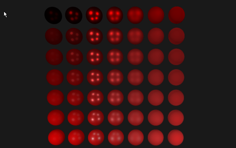
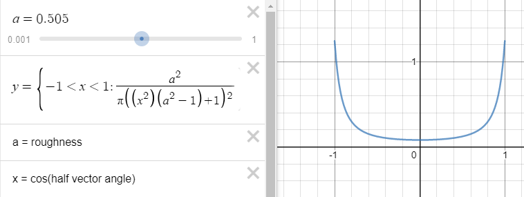
The result shown in the book is better, for a small roughness the reflections should be more point-like! In the following graph we see the Trowbridge-Reitz normal distribution function for \(a=0.505\) as a function of \(x=N.H\). For low \(a\) values the function becomes small for \(x=0\) and has large values only near \(x=1\). We should see that in our image, but no...
Now the characterisation of the material is given by textures:
uniform sampler2D albedoMap;
uniform sampler2D normalMap;
uniform sampler2D metallicMap;
uniform sampler2D roughnessMap;
uniform sampler2D aoMap;
We use the same textures as in the book of the LearnOpenGL site. They are in the folder textures/rustedIron. Using ImageMagick we can analyse the contents and we see the following: All the png files are zipped and use the sRGB space (even the normals); they all have 2048x2048 pixels; they have bit-depth=8. The normal.png has 3 channels (red, green, blue) and the albedo.png has also an alpha channel (bit-depth=1, constant value 1.0).
In most cases the albedo map is sRGBA encoded and must first be converted to linear space. This is done in the fragment shader. We load the albedo map in a RGBA texture.
Although the other files are in sRGB space we will use the values from these files uncorrected.
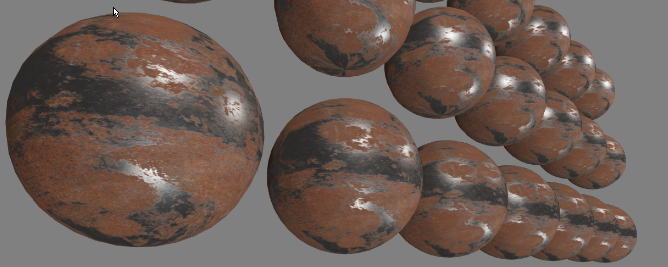
The result is seen in the following picture:
Now we use Image Based Lighting (IBL) and in this chapter we only use the diffuse part in the reflectance equation, leaving the specular part to the next chapter.
The program iblIrradiance.ts is a translation of ibl_irradianc.cpp, the program we find in the source code the book of LearnOpenGL uses. The iblCubeMap.ts is new.
In this program we load the image newport_loft.hdr (also used in the book). It is a HDR file, with light intensities larger than 1.0, that has an environment in equirectangular mapping. We convert this image to an environment in a cubemap format that also has intensities >1.0.
This program shows parts of the cubemap with intensities > 1.0. Pressing the spacebar will show the horizontal parts of the cubemap with their normal colors.
The reading of the HDR file is done with code from enkimute. The conversion to a cubemap is done using a shader that maps the equirectangular mapping to a cubemap with the use of a framebuffer. In the conversion values >1.0 must stay >1.0. For that reason we make use of a cube-texture with internal format gl.RGBA16F. To use this texture in the framebuffer (calling framebufferTexture2D) it must be color renderable. In WebGL2 it is not (https://developer.mozilla.org/en-US/docs/Web/API/WebGLRenderingContext/texImage2D), so we have to use the extension gl.getExtension("EXT_color_buffer_float") for that reason. If things go wrong look for 'framebuffer incomplete' messages.
Another technical problem is the orientation of the different faces of the cubemap, look at https://www.khronos.org/opengl/wiki/Cubemap_Texture.
In the fragment shader fs_equirectangleToCubemap we changed out uvec4 uFragColor; into out vec4 FragColor;. Otherwise the fragment shader output type does not match the bound framebuffer attachment type.
After creating the texture on all six sides of the cube we use the cubefaceShader to render the faces. The boolean uniform showIntensity determines if we see the colors or the intensities>1.0 in the result. There is also an option to look at the top and bottom faces of the cube (press key '2').
This is the translation of ibl_irradianc.cpp into javascript. It creates and uses an irradiancemap for IBL and additional four lamps. The program uses the irradiancemap only for the diffuse term.
In the same way as in the previous program the cubemap envCubemap is created from a HDR file and then this cubemap is used to create the irradiance map irradianceMap again face by face using a framebuffer.
The irradiancemap is calculated in the irradianceShader (using the glsl in fs_irradianceConvolution.js). When the cube is rendered, the position on the cube is converted to the Normal, the direction we look at, and two directions perpendicular to the normal are created with
vec3 up    = vec3(0.0, 1.0, 0.0);
vec3 right = cross(up, N);
up         = cross(N, right);
This coordinate system is used to create the hemisphere in the direction of the Normal, and characterized with a \(\phi , \psi\) as spherical coordinates. We divide the sphere in equal parts and calculate the average of the intensities in the different directions.
Note that we scale the sampled color value by cos(theta) due to the light being weaker at larger angles and by sin(theta) to account for the smaller sample areas in the higher hemisphere areas:
irradiance += texture(environmentMap, sampleVec).rgb *
cos(theta) * sin(theta);In this chapter the split-sum approximation is used, giving rise to a pre-filtered environment map (with a mipmap for a number of rougness levels) and the BRDF integration map (a 2 dimensional lookup texture with parameters roughnes and NdotV). The theory of this procedure is in the book and this is based on the description given in Epic games. In that article we find also a reason why the Geometry function is a bit different when using IBL or direct lighting.
The file readDds.ts a portion of a file with Copyright (c) 2012 Brandon Jones, for internet link and terms of use see readDds.ts
The tool cmftStudio (free software) can be used to view all kinds of maps and to convert between different formats. It can be used to read a .hdr file and to create a irradiancemap for instance. CmftStudio makes use of the DDS file format among others. This format can be used to store cube maps and textures with levels of detail. In this chapter we will create an irradiance map with a level of detail for different roughnesses. This program, ReadDds.ts, makes it possible to read these files.
The DirectDraw Surface container (DDS) file format is a Microsoft format for storing data compressed with the proprietary S3 Texture Compression (S3TC) algorithm, which can be decompressed in hardware by GPUs. This makes the format useful for storing graphical textures and cubic environment maps as a data file, both compressed and uncompressed.
The testDds is called from readDds.html.
In testDds.ts we use the extension 'WEBGL_compressed_texture_s3tc'.
This program is a part of the next (iblSpecular.ts) and creates a BRDF Lutt that is a part of the split-sum approximation. Use brdfLutt.html to start this program.
This program is the javascript translation of the C++ file ibl_Specular.cpp, used in the LearnOpenGL book.
The first part of the program is the creation of the irradiance map, the same as in Chapter 45. Then a pre-filter cubemap is created with a mipmap for a number of values for roughness. Finally a BDRFLuttMap is created as was done in brdfLutt.ts.
And now with textures on the spheres for the different materials.
This is the continuation of the GltfModel we used in project learnOpenGL2_3B. There we only loaded the meshes, now we load the materials as well.
a change to the previous version is that in the constructor of the class GltfModel the parameter useMaterials is added and the parameter is no longer found in getMeshes() and getMesh().
In the previous version of GltfLoader the images were not loaded, so the first thing we wil do is to add this functionality to the file GltfLoader.ts. After using the loader the GltfResource that we poduce must have its field images filled with all the images referenced by the model. In GltfLoader we add the fields imagesRequested and imagesLoaded and add the method
imagesComplete(resource: GltfResource): boolean {
    return (this.imagesRequested == this.imagesLoaded
    );
}
that plays a similar role as buffersComplete. In fact, the whole process of loading images and buffers is similar. We add if (gltfResource.json.images) {...} to the load(uri) method and add the loadImage, the loadImageCallback and the errorImageCallback functions that are referenced from this code block.
After the changes made to the GltfLoader we now change the GltfModel to include also materials. If useMaterials is true we create an array of GltfMaterials in the GltfModel constructor, together with a GltfTextures array (a GltfTexture has a reference to an image and to a GltfSampler) and a GltfSampler array (a GltfSampler tells how to filter and wrap the texture). These classes are in the new file geometry/GltfMaterial.ts. There we parse the information for the material in the json format we have from the the resource (that was read from file). The definition of the Gltf format for Materials can be found at the Khronos site. The format is quite complicated. The following example is from the specification:
{
    "materials": [
        {
            "name": "Material0",
            "pbrMetallicRoughness": {
                "baseColorFactor": [ 0.5, 0.5, 0.5, 1.0 ],
                "baseColorTexture": {
                    "index": 1,
                    "texCoord": 1
                },
                "metallicFactor": 1,
                "roughnessFactor": 1,
                "metallicRoughnessTexture": {
                    "index": 2,
                    "texCoord": 1
                }
            },
            "normalTexture": {
                "scale": 2,
                "index": 3,
                "texCoord": 1
            },
            "emissiveFactor": [ 0.2, 0.1, 0.0 ]
        }
    ]
}
In this example we have a baseColorTexture, a metallicRoughnessTexture and a normalTexture all having an index and texCoord. They are examples of GltfTextureInfo objects. The index is an index to the textures collection of the model. The texCoord tells which attribute we have to use, in this example TEXCOORD_1 for every texture (used as a key to the mesh.primitives.attributes).
In the program iblSpecularTextured of Ch46 we used different names for the textures.
In the GltfFile we use: * baseColorTexture instead of albedoMap * normalTexture instead of normapMap * metallicRoughnessTexture instead of two: metallicMap + roughnessMap * occlusionTexture instead of aoMap. * emissiveTexture (we did not use emission, light given off by a metarial even when there is no incoming light)
Apart from reading the values from textures the values can also be given as factors. In the example metallicFactor, emissiveFactor, baseColorFactor, roughnessFactor. In the example both a texture and a factor is used and the final value of the colors is calculated as a combination of both.
Note/warning: after the program load_Gltf_Waterbottle.ts we write the programs load_gltf_scene2.ts .. load_gltf_scene4.ts. There we introduce a glSceneManager and a glMaterialManager. That code still works but is superseded by the code in the final project (learnOpenGL2_pFinal). There we have only one GlManager class and also the shader classes work there differently. However, the texts that go with these programs still remain relevant.
In this program we will use the model waterbottle (see subdirectory models). We do it to give an example of loading a material from a gltf file. We start from a copy of the shader of the lightingTextured program of ch44 and the load_gltf.ts program of ch21.
The shader we use is made for the waterbottle alone: * Of course we use the texture WaterBottle_baseColor.png. * Also the WaterbottleNormal.png will be used. * From the WaterBottle_occlusionRoughnessMetallic.png the components Rougness and metallic are used. They are in the green and blue components. Also the red component is used as the occlusionMap. * The emissive texture is not used.
The information is passed to our shader in /shaders/1/fs_pbr.js. The following uniforms are found in the file:
// material parameters
uniform sampler2D albedoMap;
uniform sampler2D normalMap;
uniform sampler2D occlusionMetallicRoughnessMap;
//uniform sampler2D roughnessMap;
//uniform sampler2D aoMap;
We are aware of the fact that the occlusionMap could have been in a different file separate from the matallic and roughness information. In the main() function of the file we use the same variables as we are used to:
    vec3 albedo     = pow(texture(albedoMap, TexCoords).rgb, vec3(2.2));
    vec3 OMC  = texture(occlusionMetallicRoughnessMap, TexCoords).rgb;
    float metallic = OMC[2];
    float roughness = OMC[1];
    float ao        = OMC[0];
In the function resourcesLoaded() in the file load_gltf_Waterbottle.ts we load the model setting the parameter useMaterials = true. We have added the code to create gl-textures (also the samplers are loaded there). Then the bottleShader is created and is initialized with the texture units for the albedoMap, the normalMap and the occlusionMetallicRoughnessMap. Then we call createGlDrawable() to set the values of the primitives in the only mesh of the file.
function resourcesLoaded(res: GltfResource): void {
    let model = new GltfModel(res, true);
    let meshes = model.getMeshes();

    glTextures = new Array(model.textures.length);
    for (let i = 0; i < model.textures.length; i++) {
        glTextures[i] = createGlTexture(gl, model.textures[i]);
    }

    bottleShader = new Shader(gl, vs_pbr, fs_pbr);
    bottleShader.use(gl);

    bottleShader.setInt(gl, "albedoMap", TEXUNIT_ALBEDO);
    bottleShader.setInt(gl, "normalMap", TEXUNIT_NORMAL);
    bottleShader.setInt(gl, "occlusionMetallicRoughnessMap", TEXUNIT_PBR);

    if (meshes.length > 0)
        glMesh = createGlDrawable(model, meshes[0]);
    afterLoad();
}
the use of the term sampler can be confusing. In the gltf file a sampler tells us the way a texture should be filtered. After OpenGL version 3.3 a very similar object can be created, separate from the definition of a texture. It is very different from a sampler in the GLSL language. For the difference, see samplers in GLSL and Sampler objects.
We make the reasonable assumption that the texCoordinates are the same for all the textures so that in all GLSL calls to sample a texture we use texture(..., TexCoords). We do'nt use the factors (e.g. metallicFactor) that acompany the textures in the Gltf file, so that all in all we make almost no changes to the shader we already used in Chapter 44. In the shader we have four lights (as we had in Chapter 44). And this time we let the model rotate. The result is seen in the following image 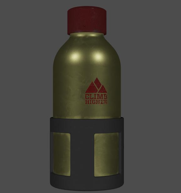 .
.
Now we rearrange the code. In this program we use the GlSceneManager class in the file glSceneManager.ts. It is used to produce the OpenGL objects needed in a scene for a model without materials. In the program of the next section, load_gltf_scene3, we add a GlMaterialManager class to produce the OpenGL objects needed for materials.
The main method of the class GlSceneManager getGlScene(glftModel: GltfModel, sceneId: number) that creates the OpenGL objects for a scene in the gltfModel i.e. the vertex buffers for the meshes in the scene. After creating a GlSceneManager we can change the field attributeLayout to reflect the positions of the attributes in the shader we use.
The GlSceneManager class (and also the GlMaterialManager class) are made in a way that makes it possible to have more than one model present in the manager class. For this we added modelName to gltfResource class, name and scenecount to gltfModel. The name of the model will be the filename of the model and the method glModelId(name) will find the index of the model within the manager.
With all this in place we can draw our cyborg again using our GlSceneManager. If we compare this program with the program load_gltf_scene of Part3, we see that a lot of the code has been transfered from the main program to the manager class.
We added the file glMaterialManager.ts. The class GlMaterialManager is responsible for creating the OpenGL objects for materials. The main method is getGlMaterialModelGltf(gltfModel: GltfModel) that first creates all the OpenGL textures and then creates a GlMaterialGltf for all the materials in the model. A GlMaterialGltf is made using a GltfMaterial found in the GltfModel, it is more or less a copy, but this time the textures are the OpenGL textures. And we have a field mapCode in GlMaterialGltf, that we will use in the shader of load_gltf_scene4. In the fragment shader the uniform albeodMap is renamed to baseColorMap. In this program we use the same shader as in the program load_Gltf_Waterbottle.ts to produce the waterbottle once again.
Now the shader program will be using the mapCode. In the new fragment shader we will use new uniforms for all the factors found in the materials:
uniform vec4 baseColorFactor;
uniform float normalScale;
uniform float metallicFactor;
uniform float roughnessFactor;
uniform float occlusionStrength;
uniform vec3 emissiveFactor;
In the Gltf specification we can find the deault values for these factors and how to combine these factors with the corresponding textures. If we look at appendix B of the specification we see suggestions for the use of the brdf functions, very similar to the formulas used in LearnOpenGL. There \(\alpha = roughness^2\) is used, but in our shader the same is done inside the function definitions.
In the models directory we have the folloowing models:
waterBottle.gltf";// scaleModel = 15.0
monster.gltf"; //scaleModel=0.1;
cyborgObjCam.gltf"; //scaleModel = 1.0
2CylinderEngine.gltf"; //scaleModel = 0.01
In our code we can use these models by out-commenting a line in load_gltf_scene4.ts and setting the variable scalemodel to the suggested values in the comment. As it is the program will show the 2CylinderEngine with scaleModel=0.01.
When we use a model without a material we have as the default values for both metallic and roughness the value 1.0. When we use the "cyborgObjCam.gltf" model the result is not pretty with these values. The result gets much nicer when setting roughness = 0.2; in our fragment shader.
Our gltf loader does handle the model and material information in the gltf file. Sometimes there is much more in the file: animations, skinning and morphing. May be we can add a Part8 to this series and add a gltf loader that does this as well, but for now this is it.
Our shader PbrShader.ts does create one OpenGL shader and it passes the mapCode to that shader. As a result of this there are a number of IF stateents in the fragment shader code like if ((mapCode & CUseBaseColorMap)>0) .... One can also opt for a solution in which a openGl shader is created for each combination of options and each shader does not have the IF-statements. The next subsection is a copy from the internet and if this is right then it seems that our solution is more simple and the harm done by the IF-staements negligable.
The following text is copied from stackoverflow.com.
What is it about shaders that even potentially makes if statements performance problems? It has to do with how shaders get executed and where GPUs get their massive computing performance from.
Separate shader invocations are usually executed in parallel, executing the same instructions at the same time. They're simply executing them on different sets of input values; they share uniforms, but they have different internal registers. One term for a group of shaders all executing the same sequence of operations is "wavefront".
The potential problem with any form of conditional branching is that it can screw all that up. It causes different invocations within the wavefront to have to execute different sequences of code. That is a very expensive process, whereby a new wavefront has to be created, data copied over to it, etc.
Unless... it doesn't.
For example, if the condition is one that is taken by every invocation in the wavefront, then no runtime divergence is needed. As such, the cost of the if is just the cost of checking a condition.
So, let's say you have a conditional branch, and let's assume that all of the invocations in the wavefront will take the same branch. There are three possibilities for the nature of the expression in that condition:
Compile-time static. The conditional expression is entirely based off of compile-time constants. As such, you know from looking at the code which branches will be taken. Pretty much any compiler handles this as part of basic optimization.
Statically uniform branching. The condition is based off of expressions involving things which are known at compile-time to be constant (specifically, constants and uniform values). But the value of the expression will not be known at compile-time. So the compiler can statically be certain that wavefronts will never be broken by this if, but the compiler cannot know which branch will be taken.
Dynamic branching. The conditional expression contains terms other than constants and uniforms. Here, a compiler cannot tell a priori if a wavefront will be broken up or not. Whether that will need to happen depends on the runtime evaluation of the condition expression. Different hardware can handle different branching types without divergence.
Also, even if a condition is taken by different wavefronts, the compiler could restructure the code to not require actual branching. You gave a fine example: output = inputenable + input2(1-enable); is functionally equivalent to the if statement. A compiler could detect that an if is being used to set a variable, and thus execute both sides. This is frequently done for cases of dynamic conditions where the bodies of the branches are small.
Pretty much all hardware can handle var = bool ? val1 : val2 without having to diverge. This was possible way back in 2002.
Since this is very hardware-dependent, it... depends on the hardware. There are however certain epochs of hardware that can be looked at:
Desktop, Pre-D3D10 There, it's kinda the wild west. NVIDIA's compiler for such hardware was notorious for detecting such conditions and actually recompiling your shader whenever you changed uniforms that affected such conditions.
In general, this era is where about 80% of the "never use if statements" comes from. But even here, it's not necessarily true.
You can expect optimization of static branching. You can hope that statically uniform branching won't cause any additional slowdown (though the fact that NVIDIA thought recompilation would be faster than executing it makes it unlikely at least for their hardware). But dynamic branching is going to cost you something, even if all of the invocations take the same branch.
Compilers of this era do their best to optimize shaders so that simple conditions can be executed simply. For example, your output = inputenable + input2(1-enable); is something that a decent compiler could generate from your equivalent if statement.
Desktop, Post-D3D10 Hardware of this era is generally capable of handling statically uniform branches statements with little slowdown. For dynamic branching, you may or may not encounter slowdown.
Desktop, D3D11+ Hardware of this era is pretty much guaranteed to be able to handle dynamically uniform conditions with little performance issues. Indeed, it doesn't even have to be dynamically uniform; so long as all of the invocations within the same wavefront take the same path, you won't see any significant performance loss.
Note that some hardware from the previous epoch probably could do this as well. But this is the one where it's almost certain to be true.
Mobile, ES 2.0 Welcome back to the wild west. Though unlike Pre-D3D10 desktop, this is mainly due to the huge variance of ES 2.0-caliber hardware. There's such a huge amount of stuff that can handle ES 2.0, and they all work very differently from each other.
Static branching will likely be optimized. But whether you get good performance from statically uniform branching is very hardware-dependent.
Mobile, ES 3.0+ Hardware here is rather more mature and capable than ES 2.0. As such, you can expect statically uniform branches to execute reasonably well. And some hardware can probably handle dynamic branches the way modern desktop hardware does.
First we give the terminology used in radiometry (in photometry they use different terminology and units for essentially the same concepts). After that we use an excercise that uses the concepts to get a feel for them.
Both radiance and irradiance are defined at a point in space, unlike flux that is integrated over an area.
For point sources we use radiant intensity, for extended sources we use radiance.
When the radiance of a source is known we can calculate the irradiance/exitance of the source by integration over a solid angle (a hemisphere). Also the flux through a surface can be calculated by integrating the irradiance over the area.
It is a theorem that radiance is conserved along points on a ray. The proof goes like this (see figure):
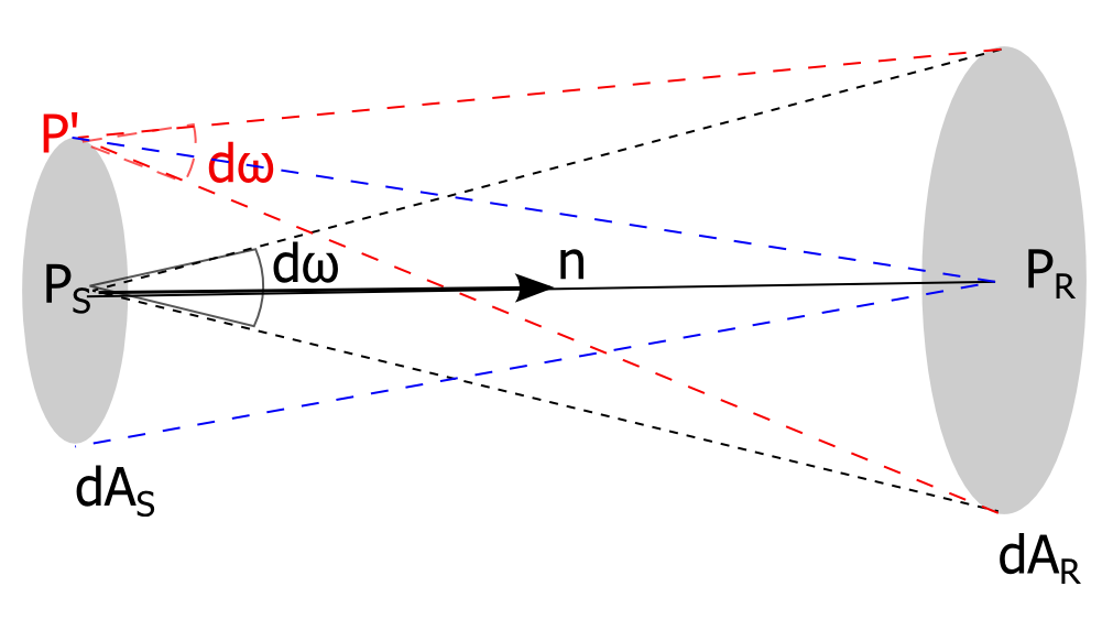
We start with an arbitrary very small area of the source (\(dA_S\)) and follow light rays that pass through this area in the direction of the receiver. First we look at the rays through \(P_S\) that are within \(d\omega\) around the normal on \(dA_S\) and see that these rays pass through an area \(dA_R\) of the receiver. Now that we have defined \(dA_S\) an \(dA_R\) we look at all the rays that go through both. If \(dA_S\) is small enough the solid angle of the 'red' rays thought \(P'\) is the same as through \(P\) and the flux \(d\Phi\) of all the rays through the area \(dA_S\) is equal to \(d\Phi = L_S.dA_S.d\omega\), where \(L_S\) is the radiance at \(P_S\). The flux that entters at \(A_S\) is the same as the flux that leaves \(A_R\). This flux at the receiver can be written in the same way as above \(d\Phi = L_R.dA_R.d\omega_R\), if we take for \(\omega_R\) the solid angle that starts in \(P_R\) and ending on the rim om \(dA_S\) (see the blue lines in the figure).
If the distance from \(P_S\) to \(P_R\) is \(d\), then we an write the following equations:
\(d\Phi = L_S.dA_S.d\omega = L_R.dA_R.d\omega_R\)
using the definition of a solid angle we have
\(d\Phi = L_S.dA_S.dA_R/d^2 = L_R.dA_R.dA_S/d^2\)
Conclusion: \(L_S = L_R\).
We started with two areas on sender and receiver that were perpendicular to the connecting ray \(P_S - P_R\), but because in the definition of radiance the measurements are always made on areas perpendicular to the rays the same argument can be made even if the areas on sender and receiver are not parallel.
Another important fact is about a Lambertian surface. Because the radiance is a constant we can give a relation between radiance and irradiance by integrating the radiance over a hemisphere: \(E = d\Phi/dA\), with \(\Phi\) the flux that goes through the hemisphere above \(dA\), with \(dA\) being a disk. Using spherical coordinates this becomes
\(E=d\Phi/dA = L \int_0^{2\pi}\int_0^{\pi/2}sin(\theta)cos(\theta)d\theta d\phi\),
\(E=2\pi \int_0^{\pi/2}sin(\theta)cos(\theta)d\theta=2\pi (1/2.sin^2(\theta))|_0^{\pi/2} = \pi L\)
A Lambertian surface is a simple example for reflexions, the outgoing reflected radiance is a constant. A less simple model uses a BRDF function, \(f_r = d L_r(\omega_r) / d E_i(\omega_i)\) where the outgoing radiance \(L_r\) is dependent on the view angle and on the angle of incoming radiance as well.
The following exercise is taken from a series of problems by Institut d'Optique – Mathieu Hebert:
Exercise 9) A is a circular disk that acts as a source with a radiance of \(10 W.sr^{-1}.cm^{-2}\) radiating uniformly in all directions toward plane BC. 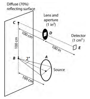
The diameter of A subtends 2° from point B. The distance AB is 100 cm and the distance BC is 100 cm. An optical system at D forms an image of the region about point C at E. Plane BC is a diffuse (lambertian) reflector with a reflectivity of 70%. The optical system (D) has a 1 \(inch^2\) aperture (1 inch = 2.54 cm) and the distance from D to E is 100 inch. The transmission of the optical system is 80%. We wish to determine the power incident on a 1- cm square photodetector at E.
Question
Determine successively: 1) the flux of the disk, 2) the irradiance at B, 3) the irradiance at C, 4) the reflected radiance at C, 5) the irradiance of the detector at E and the power received by the detector.
Solution
Flux: First we find the radius \(R\) of the disk. The distance from disk to point B, \(d_{AB}\), is given as 1 meter, so \(R=tan(1°).d_{AB}\). The area of the disk is \(\pi R^2\). Assume there is only radiation in the direction of the plane. The light is sent over a semisphere (\(2\pi\) steradent). Every \(dA\) of the disk sends \(\pi dA L_{disk}\) (not \(2\pi dA L_{disk}\), we have to correct with \(cos(\theta)\), the angle between the normal and the direction the light is sent) and the disk as a whole has a flux of \(\Phi = (\pi R^2) (\pi L_{disk})\) Watt (given is: \(L_{disk} = 10 W.sr^{-1}.cm^{-2})\). The flux sent in different directions is not the same, so do not use this source as a uniform point source.
Irradiance at B: Draw a ray from A to B. A small area round B \(dA_B\) receives from the disk a flux \(d\Phi = L_B.d\Omega_{disk}.dA_B=L_A.(\pi R^2/d_{AB}^2).dA_B\), so the irradiance is \(E_B=d\Phi/dA_B=L_A.(\pi R^2/d_{AB}^2)\), where \(d_{AB}\) is the distance from A to B.
Irradiance at C: Now the sender (the disk) and the receiver (the plane) are both at an angle \(\theta_C = \pi / 4\) with the light direction. Draw a ray from A to C. The distance \(d_{AC} = \sqrt{2}.d_{AB}\). An area \(dA_C\) at C receives the flux \(d\Phi = L_C.dA_C.cos(\theta_C).d\Omega_{disk}'= L_A.dA_Ccos(\theta_C).(\pi R^2)cos(\theta)/d_{AC}^2\), so the irradiance is \(E_C=d\Phi/dA_C = L_A.cos^2(\theta)(\pi R^2/d_{AC}^2)\).
Reflected radiance at C: The exitance at C is \(\rho.E_C\), where \(\rho\) is the reflectance = 70%. The plane is Lambertian so the radiance is constant in all directions the same, say \(L_C\). This gives an exitance \(\int_\Omega L_C cos\theta d\omega=L_C \int_\Omega cos\theta d\omega=\pi L_C\), so \(L_P=\rho.E_C / \pi\)
Irradiance at E: Take the small area \(dA_E\). The light falling in through the aperture has a solid angle \(d\Omega=dA_D/d_{DE}^2\) and the flux falling in is \(d\Phi=\tau.L_C.dA_E.dA_D/d_{DE}^2\), where \(\tau\) is the transmission of the optical system. The irradiance at E is \(E_E=d\Phi/dA_E=\tau.L_C.dA_D/d_{DE}^2\)