version 25 mei 2021; D3Q.
This article is about digital signal processing (dsp). We have applications in mind like changing the pitch of an instrument and time streching a song keeping the pitch the same. Look at this lecture to get an idea of the many ways people have come up with ideas to represent sound (and make changes to it). All the sheets in that lecture have to do with Fourier analysis and with filtering.
We will look at filters and at Fourier transforms of digital signals. The digital signals are thought to be sampled from continuous signals using a DAC (Digital-Analog-Converter). The signals are fed into systems that are supposed to be LTI (Linear-Time-Invariant) systems. Linearity means that if we feed a signal \(x_1\) into the system and the result is the signal \(y_1\), and similary if the input is \(x_2\) with the result \(y_2\), then if the input is \(\alpha x_1 + \beta x_2\) the output of the system will be \(\alpha y_1 + \beta y_2\). Time invariance means that whether we apply an input to the system now or \(T\) seconds from now, the output will be identical except for the time delay of T seconds.
We will use the symbol \(x(n)\) to denote a discrete signal and we will be thinking about this as as signal that came into being by sampling a continuous signal at equal time intervals \(T_s\) or equivalently at a constant sampling frequency \(f_s = 1/T_s\). We could have used just as well the notation \(x_n\) instead of \(x(n)\). The \(n\) is an indication of the time the sample was made.
It is not difficult to see that for LTI systems the reaction to an incoming signal is specified by its reaction to an incoming signal \(\delta(n)\), a signal that has the value \(1\) at \(n=0\) (time zero) and is zero for all other \(n\). The reason is that any signal \(x(n)\) can be written as \(\alpha_1 \delta(n) +\alpha_2 \delta(n-1)+...\), a linear combination of delta-functions and the reaction to \(\delta(n-1)\) is known if the reaction to \(\delta(n)\) is known because of time-invariance. The reaction to the signal \(x(n)=\delta(n)\) is called the impuls response and denoted by \(h(n)\). So, one way to describe a system is by giving \(h(n)\). The systems we use are called filters.
The most important theorem of sampling is the Nyquist Theorem. It states that a continuous signal that has frequencies (a Fourier transform) between \(-B\) and \(+B\) must be sampled at a frequency of at least \(2B\) if one wants to be able to recouver the original continuous signal without any loss.
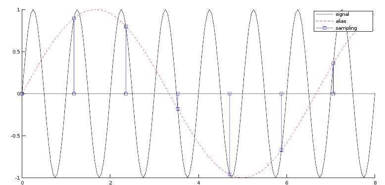
At first we might think that it will be good enough to sample with frequencies above \(B\) instead of \(2B\). The figure shows a signal of 1000 Hz during 8 msec. If a sampling frequency is used that is a little above this frequency it gives rise to a signal of low frequency (the dotted red line). In the sampling process this amplitude (of the high frequency) will be added to that low frequency, for the sampling process the two frequencies will be indistinguishable (they are an alias of each other). So, when sampling, one first chooses the highest frequency to be preserved and one chooses a Nyquist frequency above this. The sampling is done at twice this rate (\(f_s\)). Before the sampling is done an anti-aliasing filter is inserted to get rid of the frequencies above the highest frequency. As an example, humans can detect sounds in a frequency range from about 20 Hz to 20 kHz.For this reason Audio CDs have a sampling rate of 44100 samples/sec (and so, the Nyquist frequency is 22050 Hz).
The Nyquist theorem is also important when downsampling a digital signal. As a first step the high-frequency waves have to be fitered out before the actual downsampling can begin.
The examples we use are made with Octave, a free program that is something like a look-alike of Matlab. The programs we write probably work in Matlab as well. We use some of the Fourier tranforms and the Filter functions (fft, ifft, filter, freqz) and plot commands (Octave uses gnuplot to make graphics). Be aware of the fact that indices of an array start at 1 (and not 0 as in C, C#, javascript). Everything we need can be found in this manual. Chapter 31 is on the signal processing commands. When using the Windows installer Octave is installed with a nice user interface and gnuplot is installed automatically as well. There are many tutorials on the use of Matlab and Octave on the internet. Some of the programs in this file use functions found in package signal (use pkg load signal to load this package).
Especially useful is Eulers relation \(exp^{i\phi}=cos(\phi)+isin(\phi)\). Many people use the letter \(j\) instead of \(i\) for the imaginary number.
Consider \(N\) consecutive points of a signal \(x(n)\). The discrete Fourier transform (DFT) of this interval in the signal \(x(n)\) is given by the following formula:
\(X(k) = \sum_{n=0}^{N-1} x(n) e^{-i (2\pi /N)kn }\)
The inverse transform that gives us back the signal \(x(n)\) is given by:
\(x(n) = \frac{1}{N} \times \sum_{k=0}^{N-1} X(k)e^{i (2\pi /N)kn }\)
These transforms can be used for complex signals \(x(n)\) and in that case we have an input of \(N\) complex values or \(2N\) real values and the transform returns also \(N\) complex values or \(2N\) real values \(X(k)\). When the input signal \(x(n)\) is real-valued (there are no imaginary parts) then there are only \(N\) values in the input \(x(n)\) and there are also \(N\) values in the output, because then we have \(X(k)=-X^*(N-k)\), where \(X^*\) is the complex conjugate.
We see the \(N\) numbers of the time domain as the representation of the signal with \(N\) real basis-functions the \(b(n)_k=\delta(n-k)\) functions, \(0\lt k\lt N-1\). And the complex Fourier transform as the representation of the signal with \(N\) complex basis functions \(b^f(n)_k=e^{ik(2\pi n/N)}\). The real Fourier transform represents a real signal with a total of \(N\) independent real \(b^c(n)_k=cos(k*2\pi n/N)\) and \(b^s(n)_k=sin(k*2\pi n/N)\) basis functions. The Fourier coefficients are the correlation between the signal \(x(n)\) and the base functions \(b(n)_k\). After doing a complex Fourier transform on a real signal we can immediately see what the Fourier coefficients will be if we had done a real Fourier transform: we write the complex \(X(k)\), using Eulers formula, as \(X(k) = \sum_{n=0}^{N-1} x(n)( cos(2\pi kn/N)-isin(2\pi kn/N))\). So the real and imaginary parts of \(X(k)\) correspond to \(\sum_{n=0}^{N-1} x(n)( cos(2\pi kn/N)\) and \(-\sum_{n=0}^{N-1} x(n)( sin(2\pi kn/N)\). Because we have a real signal we have \(X(1)=X(N-1)\), \(X(2)=X(N-2)\) etc. only half of the base functions are independent. We have, when \(N\) is even, two special base functions that are always real themselves, for \(k=0\) and for \(k=N/2\). The first base function equals \(1\) and the second base function is the function that changes sign for every next \(n\). All the other values \(0 \lt k \lt N/2\) have a \(cos\) and \(sin\) base function, giving a total of \(N\) different base functions.
We will calculate the Fourier transform of the (very very short) complex signal \([x] = [(1.0), (2.0+1.0i), (-1.0i), (0.0) ]\)
First we do this by hand. We abbrevate \(e^{-i (2\pi /N)}\) as \(E\). And because \(N=4\) we have \(E=(-i)\), \(E^2=(-1)\), \(E^3=(i)\) and \(E^4=(1)\), so we have:
\(X(0) = x(0)+x(1)+x(2)+x(3)=(3.0)\)
\(X(1) = x(0) + x(1)E+ x(2).E^2 +x(3).E^3 = (2.0-1.0i)\)
\(X(2) = x(0) + x(1)E^2+x(2)E^4+ x(3)E^6 = (-1.0-2.0i)\)
\(X(3) = x(0)+x(1)E^3+x(2)E^6+x(3)E^9 = (3.0i)\)
These four complex amplitudes form the Fourier transform of our signal. Now we will use the fft (Fast Fourier Transform)function found in Octave. We introduce the signal over the interval having the four given values of \(x(n)\). Executing the following program
clear all;

x=[1.0+0.0i,2.0+1.0i,0.0-1.0i, 0.0+0.0i];
X=fft(x);
and asking for the contents of \(X\) gives us the same answer as done by hand. Adding the following statement:
y=ifft(X);will give back the original signal in \(y\), ifft being the inverse fft function.
We now look at a signal that is composed of one or more sine waves. Suppose the signal is sampled for a longer time and we look at the samples 1024 samples at a time. The sine completes 25 oscillations in that sampling window. Then we have: \(x(n) = sin(2 \pi \times 25n/1024)\)
Using Octave once more
clear all;

% test one sine wave
n=(0:1:1023);
s1=sin(2*pi*25*n/1024);
X=fft(s1);
plot(n,-i*X);
It produces a plot of the spectrum. Our sine wave does produce a transform with imaginary numbers (a cosine would have produced a real reansform) and that is why we multiply the transform with -i. Using \(e^{i\phi}=cos\phi + i sin\phi\) a sine wave can be written as \(sin(\phi)=-i\times (e^{i\phi}+e^{-i\phi})/2\). The following plot is produced with one peak at 25/1024 and the other at 1024-25/1024:

For real valued functions, like for instance a sine or cos wave, we always have \(X(k)=-X^*(N-k)\). All the information is in the first 1024/2 =512 complex values. They have an amplitude and a phase and in the following example we will only display these values. Also not that the horizontal axis starts at \(0\) (using a range (0:1023) in Octave) and that the first element above \(0\) is \(-i*X[1]\), the first element in the \(X\)-array (remember Octave starts indices at \(1\), not \(0\)).
In the next example we add a second sine wave and this time the wave does not have a whole number of oscillations in our sampling window of 1024 samples, in our case 8.3 oscillations.
\(x(n) = sin(2 \pi \times 25n/1024)+ sin(2\pi \times 8.3n/1024)\)
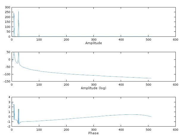
We will plot the amplitude and the phase of the Forier transform for the first 512 values using this program:
clear all;

% test simple fft
n=(0:1:1023);
s1=sin(2*pi*25*n/1024);
s2=sin(2*pi*8.3*n/1024);
X=fft(s1+s2);
XAmpl = abs(X);

subplot(3,1,1);
plot(n(1:512), XAmpl(1:512));
xlabel('Amplitude');

subplot(3,1,2);
plot(n(1:512), 20*log10(XAmpl(1:512)));
xlabel('Amplitude (log)');

XArg = arg (X);
subplot(3,1,3);
plot(n(1:512), XArg(1:512));
xlabel('Phase');
The result is:

As we can see the sine wave that does not ‘fit in our window’ also has (smaller) contributions for values on both sides of its peak. In the second figure, on a logarithmic scale, it is clear that this sine wave gives rise to contributions in all frequencies (sometimes called spectral leakage).
Often we want to find the answer to the following question: what are the frequencies in the signal at a certain time \(t_0\). To find out about the frequencies one almost alway uses the FFT algortithm. One chooses a number of samples \(N_s\) around \(t_0\) and after calculating the FFT one gets an estimation of the frequencies during that interval af time around \(t_0\), the duration being \(T = N_s*T_s\), where \(T_s\) is the time between two samples. It is not possible to find the frequency at precisely \(t_0\), we always need to use a number of samples around \(t_0\) having a duration. In the previous example we used 1024 samples having a time-span \(T\) and after using the Fourier transform, the frequencies did fall into \(512\) bins of width \(1/T\), so the frequencies in the signal also have an inprecision. And to know the time of the contributing frequencies with beter precision (making \(T\) shorter) one has to give up the precision with which the frequencies are known (the width \(1/T\) will grow). There is a trade-off between the precision of time and the precision of frequency.
Using the FFT we always first select a domain of values of \(n\) and look at the samples \(x(n)\) for those values. Before calculating the FFT we sometimes multiply the values of the samples with a window function. When this is not done (as in our previous example) one still can talk about multiplying of \(x(n)\) with a window function: in that case the window function equals \(1\) for all \(x(n)\).
We call a function \(w_L(n)\) a window function if it is zero for for all values \(n \lt 0\) and all values \(n \ge L\). \(L\) is the length of the window. The values when \(0 \lt n \lt L\) are most of the times symmetric around \(1/2 L\). When all the non-zero values are equal to \(1\) it is called a rectangular window, but there are many other window functions defined, each with its own characteristics. Almost always these functions tend to zero at both edges and have a maximum in the middle. An example is the Hann window function. The formula for this window is \(w(n)=1-0.5(1-cos(2\pi n/N))\). Using the hann function in Octave:
clear all;

n=(0:1:1023);
win = hann(1024);
subplot(1,1,1);
plot(n, win);
xlabel('Hanning window');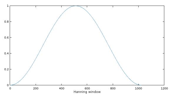
In Matlab there is a small difference between the function hann() and hanning() as to the first and last values to be zero or not. In Octave the function hann(6) and hanning(6) both will give us 6 values, the first and the last of which are 0.
Let us plot the same frequencies as above, but now with first multiplying \(x(n)\) with the Hanning window:
clear all;

% test simple fft with Hann window
win = hann(1024);

n=(0:1:1023);
s1=sin(2*pi*25*n/1024);
s1Hann=transpose(win).*s1;
s2=sin(2*pi*8.3*n/1024);
s2Hann=transpose(win).*s2;

X=fft(s1Hann+s2Hann);
XAmpl = abs(X);

subplot(3,1,1);
plot(n(1:512), XAmpl(1:512));
xlabel('Amplitude');

subplot(3,1,2);
plot(n(1:512), 20*log10(XAmpl(1:512)));
xlabel('Amplitude (log)');

XArg = arg (X);
subplot(3,1,3);
plot(n(1:512), XArg(1:512));
xlabel('Phase');
The result is now:
As expected, the sine that fits in the window is no longer a sharp line but now also has a certain width. The sine that does not fit in the window still has effects in all other frequencies, but with smaller amplitudes. The Hann(ing) window function ‘forces all sine waves to fit the window’.
Selecting a window function is not a simple task. To choose a window function, you must have a certain effect in mind. For instance we have the situation in which two very close one to another frequencies are expected and we want to see them as separate frequencies in our spectrum (we ask for a good frequency resolution). Or for instance a very small amplitude of a certain frequency is expected that might get hidden in the contributions of stronger frequencies to all frequency bins. Then we can choose different windowing functions that give us the desired effect. Octave has several function allready defined for us. The difference between them is that one window function has a smaller peak and another window function starts off from both sides faster. The general shape of all of them is the same. With no effect in mind the Hanning (Hann) window is satisfactory in 95 percent of all cases. It has a good frequency resolution and, as we saw, a reduced spectral leakage.
A Fourier transform related to the DFT is the DTFT, the discrete-time Fourier transform. It also is about discrete signals, but now all the samples in the signal are considered. It is in fact the limit of a DFT, making the number of samples, \(N\) bigger and bigger. As we have already seen, the frequency resolution will get better and better and in the limit we have:
\(X(\omega)=\sum_{-\infty}^{\infty} x(n)exp^{-in\omega}\)
\(x(n) = (1/2\pi) \int_{<2\pi>} X(\omega)exp^{in\omega}d\omega\)
Because \(X(\omega)\) is periodic in \(\omega\) we an choose any integration domain with length of \(2\pi\). Some prefer \(0<\omega<2\pi\) others \(\pi<\omega<\pi\).
As a very simple example of the DTFT we use a signal \(x(n)=\delta(n-1)+\delta(n+1)\). In that case \(X(\omega)=exp^{-i\omega}+exp^{i\omega}=2cos(\omega)\). If we have the more general signal \(x(n)=\delta(n-m-1)+\delta(n-m+1)\) then we have \(X(\omega)=exp^{-i\omega(m+1)}+exp^{-i\omega(m-1)}=2exp^{-im\omega}cos(\omega)\), a cosine function for the amplitude together with with a phase function \(exp^{-im\omega}\). This transform gives us no information about the time when we have a frequency \(\omega\).
When we have a signal that is changing in time we often use a short-time Fourier transform (STFT) that has overlapping windows. The first window starts at \(n=0\) and ends at \(n=L\) and a Fourier transform is calculated for the product of the window and the signal. Then the window is moved so that is starts at \(n=h\) and ends at \(n=L+h\) and a new Fourier transform is calculated. And so on. The value \(h\) is called the hop length. And the result is a set of spectrums in time (at \(hn\) time units apart). This result is called a spectogram. Common hop lenghts are \(0.25*L\), \(0.5*L\) and \(L\), if we want to call \(L\) a hop length at all. Some use a hop length of only one sample. In that case it is perhaps better to use the sliding fourier transform algorithm instead of the FFT to calcuate the Fourier transform.
Mathematically the STFT of a signal \(x(n)\) is given by:
\(X(\omega_{k}, m) = \sum_{n=-\infty}^{\infty} w(mh-n)x(n)exp^{-i\omega_{k}n}\), where \(\omega_{k}=(2\pi/N)k\)
For every increase of the integer \(m\) we have made a new hop. And the summation is from \(n=-\infty\) to \(n=+\infty\), because the window function will be zero, except for N values. A special example of a STST is the Gabor transform. In the Gabor transform we use a Gaussian window.
When having a spectogram, in many cases we can find the original signal back using an inverse STFT algorithm. For every value of \(m\) we can use the inverse Fourier transform to get the values of the function \(w(mh-n)x(n)\), and from that we can reconstruct \(x(n)\) in the range where \(w(n)\) has an inverse.
For certain windows there is an easy way to reconstruct \(x(n)\) with the overlap-add method. To give an impression of the overlap-add method we have the following Octave program:
clear all

N=64;

% create a signal s
% start and end of signal is zero (s0)
seq=(0:N-1);
s0=seq*0;
s2=sin(seq*2*pi*25/N);
s3=sin(seq*2*pi*8.3/N);
oldsignal=[s0,s2,s3,s0];

% signal analysis
spectgram=[];
win = hann(N+1);
whan=win(1:N);
whan=whan';

hopsize=N/4;
for hops = 0:12
  sselect = oldsignal(hops*hopsize+1:hops*hopsize+N);
  swin = whan.*sselect;
  spectgram=[spectgram; fft(swin)];
  end;

% signal manupilation
% -- omitted

% signal synthesis
newsignal=[s0, s0, s0, s0];
for hops = 0:12
  sinverse = ifft(spectgram(hops+1,:));
  newsignal(hops*hopsize+1:hops*hopsize+N)=newsignal(hops*hopsize+1:hops*hopsize+N)+sinverse;
  end;
newsignal = 0.5*newsignal;

% calc difference
diff = 0;
for i=1:4*N
    diff = diff+abs(abs(oldsignal(i))-abs(newsignal(i)));
  end;
In the program a signal is created and a number of FTT-operations is performed on 64 samples, with a hop length of 64/4=16 samples. Use is made of a hann window. The intersesting part is the recovery of the original signal from the created spectogram. The inverses of the spectrums is found with the ifft function and added to the signal, without taking the inverse of the hann window-function, even when the ifft delivers sample values of \(swin = whan*sselect\). The reason is that a hann window function has the property that when we add a sample at \(n=\delta\) and the same sample at \(n=0.5*N+\delta\) we get as a result the sample value, because the hann window is a cosine function. Because we add a sample value four times (at four different window values), the result will be twice the sample value and we have to compensate for this (\(newsignal = 0.5*newsignal;\)).
Often only getting the original signal back is not interesting. Before recovering a signal one wants to apply changes in the frequency domain. But in that case we have to be aware that changes to a STFT will not alway result in a well defined signal. As an example: we have 3 consecutive spectra in a STFT and in the frequeny domain we change the first and third to zero and leave the middle specrum as it is. If there are overlapping windows then we are left with a STFT that does not represent a signal. In that case we can only calculate a time-signal that in some way is closest to the STFT repesentation. The Griffin algorithm does this and uses the least-squares method as a measure for distance of signals.
As a closing remark we note that there is also a filter-bank interpretation of the STFT. Our next section will be on filters. At the end we come back to that interpretation.
The specification of a filter is almost always done in the frequeny domain. For example one might think of an ideal filter that lets through all the frequencies between 20Hz and 20kHz and removes the other frequncies. Ideal filters are however not realizable and the specification will have to be more complex. The terms used in a specification are seen in the following diagram:
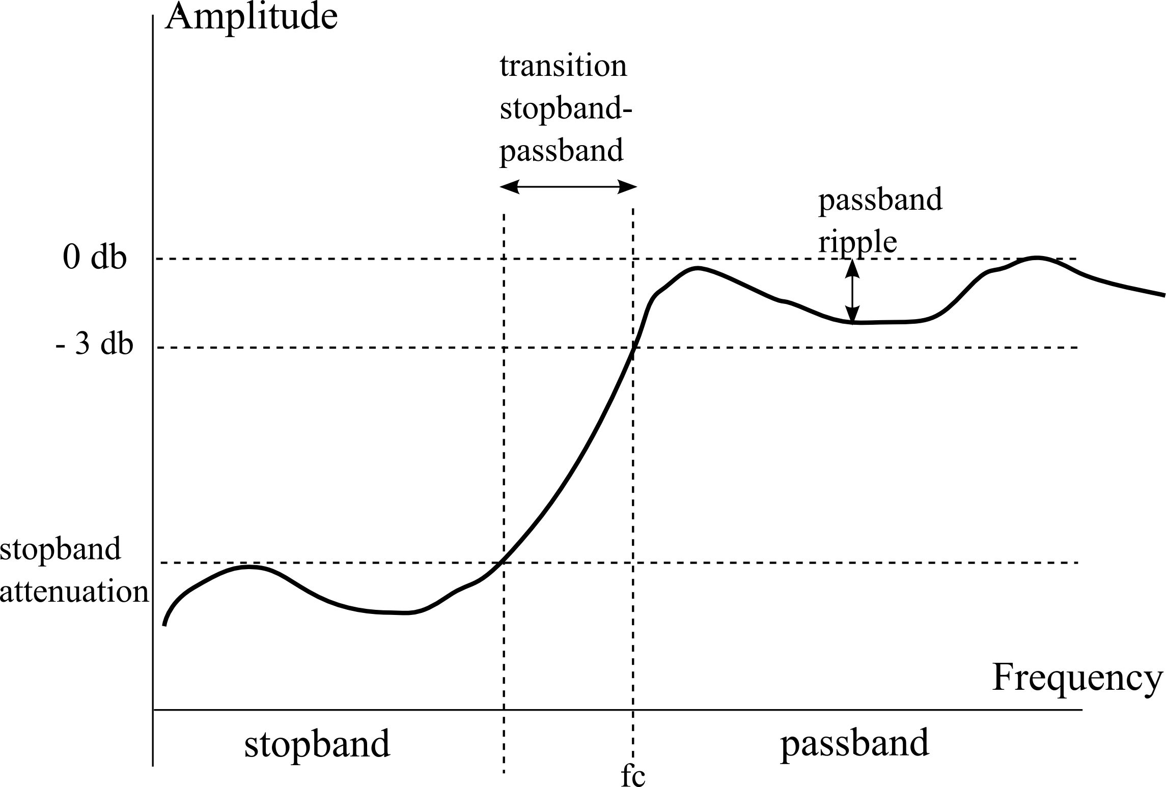
In the figure we see a high-pass filter. Important in a specification are the amount of attenuation that a stopband must have, of course also the frequncies of both the stopband and the passband are important as is the amount of ripple the passband is allowed to have. To define the width of the passband we can use the cutoff frequency, often defined as the frequency at which the output signal has one-half the power of the input signal. For the width of the stopband we can use the frequency at which the response becomes higher than the allowed attenuation.
When talking about analog filters made in hardware the input impedance and output impedance are also very important: they should match the impedance of whatever is connected to it. Digital filters can be realized using N memory locations (N taps) that hold the last N inputs and using amplifiers after the current input and after the N taps. We only look at digital filters realized in software. And we only look at one-dimensional filters.
A FIR filter is described by the following equation where the output of the filter, \(y(n)\) is given by the inputs \(x(n)\) at equal or earlier times:
\(y(n) = \sum_{k=0}^P b(k)x(n-k)\) or \(y(n) = \sum_{k=0}^P b_kx(n-k)\)
The following picture shows a discrete-time FIR filter of order N. The top part is an N-stage delay line with N + 1 taps. Each unit delay is a \(z^{−1}\) operator in Z-transform notation.
 figure FIR filterby BlanchardJ
In a IIR filter there are also feedback terms: \(y(n)\) depends on earlier outputs as well. The term \(a(0)\) is most of the times equal to one:
\(a(0)y(n) = \sum_{k=0}^P b(k)x(n-k) - \sum_{k=1}^Q a(k)y(n-k)\)
 figure IIR filter by BlanchardJ
As a very simple example we use the FIR filter \(y(n) = x(n)+ 2*x(n-1)+x(n-2)\).
Let us first look at the impulse response, i.e. the reaction of this filter on an input \([x] = \delta(n) = [...0.0, 0.0, 1.0, 0.0, 0.0, ...]\). The signal is \(1.0\) at \(n=0\) (\(t = 0*T_s'\)) and the next table shows the value of the input, memory-locations (M1 is used instead of x(n-1), M2 instead of x(n-2)) and output.
| x(n) | M1 | M2 | y(n) =x(n)+2*M1+M2 |
|---|---|---|---|
| x(0)=1 | 0 | 0 | y(0) = \(1*1+2*0+1*0\) =1 |
| x(1)=0 | 1 | 0 | y(1) = \(1*0+2*1+1*0\) =2 |
| x(2)=0 | 0 | 1 | y(2) = \(1*0+2*0+1*1\) =1 |
The output signal, the impulse response, in this case \([1, 2, 1, 0 ...]\), is in most textbooks represented by \(h(n)\). The length of the input response is three because the filter has two taps, for the rest of the time the output is zero. The word tap reminds us of how a digital filter can be constructed using a memory location plus amplifier. From now on we will use the word order that tells us what the value of \(P-1\) is in the filter equation.
Next let us look at the behaviour of this filter when it is fed with a sine wave signal \(x(n)=sin(2\pi f/f_s *n)\), where \(f_s\) is the sampling frequency. If \(f=f_s\) each increment of \(n\) will advance the sine over a full period. We are interested in all values of \(f<f_s/2\).
Instead of using the sine function we use the (imaginary part) of the complex function \(x(n) = exp(i*2\pi f/f_s *n)\). Substituting this in our filter equation we have
\(y(n) = exp(i*2\pi f/f_s *n) + 2*exp(i*2\pi f/f_s *(n-1))+ exp(i*2\pi f/f_s *(n-2))\), or
\(y(n)= x(n)*(1 +2*exp(-i*2\pi f/f_s) + exp(-2i*2\pi f/f_s)\)
Writing \(Z=exp(i*2\pi f/f_s)\) this can be written as \(y(n) = x(n)*\sum_{m=0}^2 b(n)Z^{-n}\) The ratio \(H(f)=y(n)/x(n)\) is called the system function.
If we have two signals \(x(n)\) and \(y(n)\) then the convolution of both is defined as \(x(n)\star y(n)= \sum_{m=-\infty}^{+\infty}x(m)y(n-m)\).
As mentioned before, if we have a LTI system then it can be described by its reaction \(h(n)\) to an input \(\delta(n)\). The reaction of that system to an arbitrary input \(x(n)\) will be the convolution of \(x(n)\) with \(h(n)\): \(y(n) = \sum_{m=-\infty}^{+\infty} h(m) x(n-m)\). Another way to look at this equation for LTI systems is as an operator equation: \(y(n)=O(x(n))\), which raises the question of this operator \(O\) having eigenfunctions and eigenvalues. By substitution of \(x(n)=e^{sn}\) we have \(y(n)=\sum_{m=-\infty}^{+\infty} h(m) e^{s(n-m)}=e^{sn}.\sum_{m=-\infty}^{+\infty} h(m) e^{s(-m)}=\lambda x(n)\). So \(x(n)=e^{sn}\) is an eigenfunction of \(O\) and the eigenvalue is \(\lambda = \sum_{m=-\infty}^{+\infty} h(m) e^{-sm}\). The eigenvalues as a function of \(s\) form the system function we used in the previous paragraph: \(\lambda(s)=H(s)\) and \(h(m)\) and \(H(s)\) are alternative forms to describe a LTI system.
If we have a signal \(x(n)\) then the (one-sided) Z-transform of the signal is defined as: \(Z(x(n))= \sum_{n=0}^{\infty} x(n)z^{-n}\).
The Z-transform is a mapping from the space of discrete-time signals \(x(n)\) to the space of functions defined over (some subset of) the complex plane (the ‘z’-plane). The Z-transform has a reverse transform.
If we define \(H(s)\) also for complex \(s\) then we see that \(H(z)=Z(h(n))\), so \(H(z)\) is the z-transform of \(h(n)\).
Examples of Z-transforms: 1. \(x(n)=\delta(n)\) has \(Z(x(n))=1\) 2. \(x(n)=\delta(n-k)\) has \(Z(x(n))=z^{-k}\) 3. \(x(n)={-5, 6^*, 0, 4}\) has \(Z(x(n))=-5z+6+4z^{-2}\) In this example the \(6\) has a star to indicate that \(x(n)\) has this value at index 0. 4. \(x(n)=\frac{3}{5}^n\ u(n)\) has \(Z(x(n))=1/(1-\frac{3}{5}z^{-1})\) Here \(u(n)\) has the value 1 for all \(n \ge 0\). The Z-transform is the sum of a geometric sequence.
Of course we have to know what the region of convergence (ROC) of the Z-transform is. In the last example the ROC is \(|z| \gt 2/3\). The signal with the same transorm but with ROC \(|z| \lt 2/3\) is a different signal
Some properties of the Z-transform: 1. linearity: \(Z(x(n)+y(n))=Z(x(n))+Z(y(n))\) 2. time-delay: \(Z(x(n-k))=Z(x(n)).z^{-k}\) 3. convolution: \(Z(x(n)\star y(n))=Z(x(n))Z(y(n))\) 4. multiply by n: \(Z(nx(n))=z\ \partial Z(x(n))/\partial z\)
We continue with finding the system function for a IIR filter, giving the difference equation of the filter. When using a IIR filter the length of the inpuls response can become infinite long because of the feedback terms. We start with a simple one, a first order IIR filter given by:
\(y(n) = x(n) + 2*x(n-1) -a(1)*y(n − 1)\)
Here the current output can be written in terms of the current input, the immediate past input and the immediate past output. Let us look again at the impulse response. We use Mx for the memory value of the input x(n-1) and My for the memory value of the past output y(n-1). As coefficient of the output memory we use a(1) instead of a given value, so we can see what happens for different values of a(1):
| x(n) | Mx | My | y(n) =x(n)+2*Mx+My |
|---|---|---|---|
| x(0)=1 | 0 | 0 | y(0) = \(1*1+2*0+a(1)*0\) =1 |
| x(1)=0 | 1 | 1 | y(1) = \(1*0+2*1+a(1)*1\) =\(2+a(1)\) |
| x(2)=0 | 0 | \(2+a(1)\) | y(2) = \(1*0+2*0+a(1)(2+a(1))\) = \(2a(1)+a(1)^2\) |
| x(3)=0 | 0 | \(2a(1)+a(1)^2\) | y(3)=\(1.0+2*0+a(1)(2a(1)+a(1)^2)=a(1)^2(2+a(1))\) |
…
We see that we now have a series that does not end. Every new value of \(y(n)\) will have the value \(-a(1)*y(n-1)\). And the value will become infinite in time when \(a(1)\gt 1\).
Next let us look at the behaviour of this filter when it is fed with a sine wave signal \(x(n)=sin(2\pi f/f_s *n)\).And again, instead of using the sine function we use the (imaginary part) of the complex function \(x(n) = exp(i*2\pi f/f_s *n)\).
We want to express \(y(n)\) in terms of the input \(x(n)\). Using the letter \(Z\) again as a shorthand for \(Z=exp(i*2\pi f/f_s)\) we have for instance \(x(n)=Z^n\), \(x(n-1)=x(n)(1/Z)\) and \(3=3x(n)(1/Z)^n\)
We start the signal at \(n=0\) and assume \(x(-1)=0, y(-1)=0\). Using our filter equation we can write for \(y(0),\ y(1),\ y(2),\ y(3)\) the values in terms of \(x(n)\):
\(y(0)=x(0)+2x(-1)-a(1)y(-1)=1\)
\(\begin{array} {lcl}y(1) & = &x(1)+2x(0)-a(1)y(0)\\ & = & x(n)(1/Z)^{n-1}+2x(n)(1/Z)^n-a(1)\\ & = & x(n)(1/Z)^{n-1}(1+2/Z) - a(1)\end{array}\)
\(\begin{array} {lcl}y(2) & = &x(2)+2x(1)-a(1)y(1)\\ & = &x(n)(1/Z)^{n-2}+2x(n)(1/Z)^{n-1}-a(1)\{x(n)(1/Z)^{n-1}(1+2/Z) - a(1)\}\\ & = &x(n)(1/Z)^{n-2}(1+2/Z)-a(1)(x(n)(1/Z)^{n-1}(1+2/Z))+a(1)^2 \end{array}\)
\(\begin{array} {lcl}y(3) & = & x(3)+2x(2)-a(1)y(2)\\ & = & x(n)(1/Z)^{n-3}+2x(n)(1/Z)^{n-2}-a(1)\{\\ & &\ x(n)(1/Z)^{n-2}(1+2/Z)-a(1)(x(n)(1/Z)^{n-1}(1+2/Z)+a(1)^2\}\\ & = &x(n)(1/Z)^{n-3}(1+2/Z)-a(1)x(n)(1/Z)^{n-2}(1+2/Z)+a(1)^2x(n)(1/Z)^{n-1}(1+2/Z)-a(1)^3\end{array}\)
We see a geometric sequence appearing where the terms have a common ratio \(a(1)Z^{-1}a(1)Z\)
\(y(n)= (1+2Z)\sum_{m=0}^{n-1} x(n)(-a(1)^mZ^m) + (-a(1))^n\)
Taking the sum for large \(n\), assuming convergence when \(a(1)\lt 1\) the sytem function is:
\(H(f) = y(n)/x(n)=(1+2Z^{-1}) /(1+a(1)Z^{-1})\)
To investigate the behaviour of a rational function we look for the poles and zeros. To do this one writes the nominator and denominator as a product of terms \((z-z_0)\), in this case:
\(H(f) = (1+2/Z)/(1+a/Z) = (Z+2) / (Z+a)\)
having a zero at \(Z=-2\) and a pole at \(Z=-a\).
(from http://www.eecs.umich.edu/courses/eecs206/archive/spring02/notes.dir/iir4.pdf)
\(y(n) = b(0)x(n) + a(1)y(n − 1) + a(2)y(n − 2)\)
In this equation we have real coefficients \(b(0),\ a(1), \ a(2)\)
The system function \(H(f)\) will be
\(\begin{array} {lcl} H(f) & = & b(0)/\{1-a(1)Z^{-1}-a(2)Z^{-2}\}\\ & = & b(0)Z^2/\{Z^2-a(1)Z-a(2) \}\end{array}\)
The denumerator is written as \((z-p_1)(z-p_2)\), with \(p_1p_2=-a(2)\) and \(p1+p2=-a(1)\) and because \(a(1), \ a(2)\) are real numbers the poles can be written as \(p_1=r\ exp^{+i\phi}, \ p_2=r\ exp{-i\phi}\), so:
\(\begin{array} {lcl}H(f) & = & b(0)Z^2 / \{Z-rexp^{i\phi})(Z-rexp^{-i\phi})\}\\ & = & b(0)/\{1-2rcos(\phi)Z^{-1}+r^2Z^{-2} \} \end{array}\)
Stability requirement: The two poles must reside inside the unit circle \(|r| < 1\). In the following figure we have plotted, using the Octave freqz function, the frequncy response for \(z=exp^{i2\pi f/f_s n}, 0\lt n\lt 1001\) for a filter having \(r=0.95, \phi=\pi/4\)
r =0.95;
phi= pi/4;

b = [0.125];
a = [1, -2*r*cos(phi), r*r]

[h,w] = freqz(b,a, 1001);

%Plot the magnitude response expressed in decibels.

plot(w/pi,20*log10(abs(h)));
axis ([0 1 -30 10])
xlabel('Normalized Frequency (\times\pi rad/sample)');
ylabel('Magnitude (dB)');
The result is a simple band-pass filter. The peak is for a normalized frequency equal to \(\pi/4\). Making \(r\) smaller will result in a less steep curve.
In Octave there is a function \(y = filter (B, A, x)\). Here \(x\) is the input signal (a vector of any length) and \(y\) is the output signal after filtering \(x\) with a filter giving by the coefficients \(A\) and \(B\) (\(A\) is a vector of filter feedback coefficients, \(B\) is a vector of filter feedforward coefficients)
A filterbank is an array of bandpass filters that separates the input signal into multiple components, each one carrying a single frequency sub-band of the original signal.
As an example we can use as input a chirp signal; a chirp signal is generally defined as a sinusoid having a linearly changing frequency over time: \(x(t)=cos(\theta_t)\) with \(\dot \theta_t = \alpha t+\beta\), so the frequency gets higher and higher.
The following code … TODO more text; also short time fourier transform and filterbanks (first hetreodyning with \(e^{-nf})\) and using a window as lowpass filter…
clear all;
N=10; % number of filters = DFT length
fs=1000; % sampling frequency (arbitrary)
D=1; % duration in seconds
L = ceil(fs*D)+1; % signal duration (samples)
n = 0:L-1; % discrete-time axis (samples)
t = n/fs; % discrete-time axis (sec)
x = chirp(t,0,D,fs/2); % sine sweep from 0 Hz to fs/2 Hz
%x = echirp(t,0,D,fs/2); % for complex "analytic" chirp
x = x(1:L); % trim trailing zeros at end
h = ones(1,N); % Simple DFT lowpass = rectangular window
%h = hamming(N); % Better DFT lowpass = Hamming window
X = zeros(N,L); % X will be the filter bank output
subplot(N+1, 1, 1);
plot(n, x);
for k=1:N % Loop over channels
wk = 2*pi*(k-1)/N;
xk = exp(-j*wk*n).* x; % Modulation by exponential
X(k,:) = filter(h,1,xk);
subplot(N+1,1,k+1);
plot(n, X(k,:));
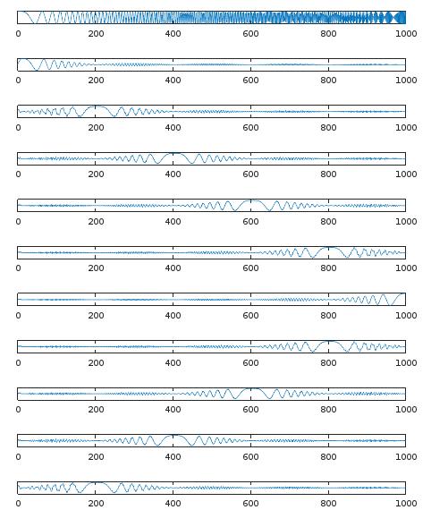
endThe result is seen in the following figure. The first graph is the chirp signal. The following 10 graphs give the signal in the ten frequency subbands.
Class notes on digital filter responses. Difference equations and the Z-transform.
This site of the Uva has pages on the Fourier transform, the Laplace transformation and the -transformation. Also some notes on the use of Python for signal processing.
The Large Time/Frequency Analysis Toolbox (LTFAT) is a Matlab/Octave toolbox for working with time-frequency analysis and synthesis. It is intended both as an educational and a computational tool. The toolbox provides a large number of linear transforms including Gabor and wavelet transforms along with routines for constructing windows (filter prototypes) and routines for manipulating coefficients.
A pdf file from the Tue on the STFT and inverse. Also treats the filterbank interpretation, the Gabor transform and the Griffin inverse STFT.
At https://www.dsprelated.com/ there are a number of free books on digital signal processing. The spectral audio signal processing (saps) book has many pages on filters, filter banks, fourier transforms, windows. At the end there are are examples in Matlab/Octave (creating a spetrogram , fundamental frequency, ) and a section on Spectral Audio Modeling. One of the chapters is devoted to the OLA inverse STFT. Another book on dsp has the same subjects: filters, windows, fourier transforms. Many chapters, not all of them are finished (chapters 30 and following). Two interesting chapters on DSP (digital signal processors).
In this pdf a nice overview of the different ways a LTI system can be described. They also mention a System Functional \(H(R)=1/(1-R-R^2)\) to describe the system. It is simply translating the output signal of the block diagram as \(Y=(X+R^2 Y+RY)\).
http://www.panix.com/~jens/pvoc-dolson.par describes a vocoder as a filterbank using the hetrodyne technique
A number of audio projects at columbia.edu. https:// And a number of Matlab projects at columbia.edu.
Here we mention a number of sites on the subject of changing the pitch of a voice and time stretching a song.
An article on Pitch shift. It uses STFT and a theory on the ‘true’ frequency to change the pitch. The true frquency is found using phase differencies. After finding the true freqencies the pitch shift is done. Then the phases are recalculated and an inverse STFT.
An other source for changing pitch is a documentation file that goes with the soundtoch library. The algorithm works primarily in the time domain. The time signal is split in short sequences with overlap and later joined together adding or leaving out some frames. The main task for a good quality is to look for a good division of the signal in sequences. The article also mentions the FFT approach called Phase Vocoder, that resembles the first article above on Pitch shift. At the library site are some audio examples. Published under the GNU Lesser General Public License version 2.1. The well known free program Audacity makes use of it (see the lib-src directory of Audacity).
A newer technique seems to be Subband Sinusoidal Modeling Synthesis (SMBS). Also used in Audacity. An application/library can be downloaded here and here, but it is not Windows-oriented. A description of Spectral Modeling Synthesis introduces a model for separately modelling the Sines + Noise + Transients (S+N+T). The general problem being that transients and noise are difficult to represent in frequency space. Also look at the PARSHL program for tracking spectral peaks in the Short-Time Fourier Transform.
In this thesis work is done on connecting one song with another song from a database. All kinds of algorithms are used.
At this site is a matlab implementation of changing the pitch made by D. P. W. Ellis. The code consists of a four files and is written in 2002. Nice code that also shows how reading and writing .wav-files can be done. In the following example the pvoc.m code is used to stretch the sound, keeping the pitch. Audioread is used to read the file ‘clar.wav’ (audioread replaces the older wavread function). Pvoc is a function made by Ellis. And the function sound plays the loaded song, first the original and then the changed version:
% pkg load signal, if not already loaded...
clear all;

[d,sr]=audioread('clar.wav');
% 1024 samples is about 60 ms at 16kHz, a good window
y=pvoc(d,.75,1024);
% Compare original and resynthesis
sound(d,16000);
sound(y,16000);